The ‘Odd’ Obsession with Odds Ratios: Making a Case for Marginal Effects in Health Research
marginal effects
Marginal Effects >>> Odds Ratios
Author
Jacob Jameson
Published
September 1, 2023
Odds ratios have been a long-standing mainstay in health research. Their use can be found sprinkled throughout countless academic journals and research papers. But just because something is popular doesn’t mean it’s the best choice for all contexts. The purpose of this article is to shed light on the limitations of odds ratios, particularly when it comes to interpretation, and advocate for the more intuitive marginal effects and predicted probabilities.
The math behind odds ratios
To understand why odds ratios can be confusing, let’s briefly discuss what they represent.
In a logistic regression, the fundamental equation is:
Where \(p\) is the probability of an event occurring.
The odds ratio for a given predictor (let’s say \(X_1\)) is simply the exponentiated coefficient for that predictor:
Odds Ratio for \(X_1 = E^{\beta_1}\)
It represents the multiplicative change in the odds of the outcome for a one-unit increase in \(X_1\) , holding other variables constant. If this sounds confusing, you’re not alone.
When Odds Ratios Mislead
The challenge with odds ratios arises particularly when the outcome of interest is common. The reason being, odds ratios tend to exaggerate relative risks for common outcomes.
Let’s say we find an odds ratio of 2 for a drug reducing heart attack risk. Many might (mistakenly) interpret this as “patients on the drug are twice as likely to avoid heart attacks.” In reality, they have twice the odds, which doesn’t translate directly to actual probabilities, especially when the event is common.
Marginal Effects: Clarity over Confusion
Marginal effects shine where odds ratios falter. They convey the change in the probability of an outcome for a one-unit change in the predictor, holding other variables constant. It’s a direct measure that offers a tangible understanding of impact.
Mathematically, for a binary predictor (like drug use: yes or no):
For continuous predictors, the marginal effect represents the derivative of the probability with respect to the predictor, which essentially gives us the rate of change.
Predicted Probabilities: Concrete Scenarios Over Abstract Odds
Predicted probabilities go a step further, providing the likelihood of an outcome under specific conditions. Instead of leaving things in the realm of odds and abstract increases, we can state tangible scenarios.
Demonstrating with “Real-World” Data
To provide concrete evidence of the limitations of odds ratios, let’s explore a simulated dataset that mirrors a health study on heart attacks, age, and drug use for high-risk individuals.
First, we’ll generate a dataset with age as a continuous predictor and drug_use as a binary predictor:
Simulate data
Show the code
# Setting the seed for reproducibilityset.seed(1234)n <-1000# Age distribution: Normally distributed between 40 and 70age <-rnorm(n, 55, 7.5)# Drug use: 50% of the participants use the drugdrug_use <-rbinom(n, 1, 0.5)# Log odds of heart attack: Base risk, then increasing slightly with age, # and decreasing with drug use (this is where we're setting the odds ratio to roughly 2 for drug use)log_odds_heart_attack <--2+0.04* age -log(2) * drug_use# Converting log odds to probabilityprob_heart_attack <-exp(log_odds_heart_attack) / (1+exp(log_odds_heart_attack))# Simulating whether a heart attack occurs or notheart_attack <-rbinom(n, 1, prob_heart_attack)# Create a dataframedata_high_risk <-data.frame(age, drug_use, heart_attack)
nrow(data_high_risk)
[1] 1000
data_high_risk
age
drug_use
heart_attack
45.94701
0
1
57.08072
0
1
63.13331
1
0
37.40727
1
0
58.21844
0
1
58.79542
1
0
50.68945
1
0
50.90026
0
0
50.76661
1
0
48.32472
0
1
Modeling and Results
Using a logistic regression, we’ll model the probability of a heart attack based on age and drug use:
model_high_risk <-glm(heart_attack ~ age + drug_use, data=data_high_risk, family = binomial)summary(model_high_risk)
Call:
glm(formula = heart_attack ~ age + drug_use, family = binomial,
    data = data_high_risk)

Deviance Residuals:
   Min      1Q  Median      3Q     Max
-1.662  -1.049  -0.854   1.188   1.685

Coefficients:
            Estimate Std. Error z value Pr(>|z|)
(Intercept) -2.24031    0.49848  -4.494 6.98e-06 ***
age          0.04281    0.00896   4.777 1.78e-06 ***
drug_use    -0.66254    0.13064  -5.072 3.94e-07 ***
---
Signif. codes:  0 '***' 0.001 '**' 0.01 '*' 0.05 '.' 0.1 ' ' 1

(Dispersion parameter for binomial family taken to be 1)

    Null deviance: 1373.7  on 999  degrees of freedom
Residual deviance: 1324.4  on 997  degrees of freedom
AIC: 1330.4

Number of Fisher Scoring iterations: 4
Upon examining the output, you’ll observe an odds ratio close to 2 for drug use (exponentiate the coeffecient). A common misinterpretation might be: “Patients on the drug have twice the likelihood to avoid heart attacks.” This is a misconception. They have twice the odds, not twice the probability. This distinction becomes especially murky when the event (heart attack) is common.
Marginal Effects and Interpretation
The marginal effect of the drug can be found by computing the difference in predicted probabilities between drug users and non-users, holding other variables constant. This gives a more direct measure of the drug’s impact on the probability of heart attack.
Using our model, you can compute the marginal effect for any given age. For example, for someone aged 55:
The result is a clear percentage point decrease in the probability of a heart attack for drug users compared to non-users.
This means that, for individuals aged 55, using the drug results in a 16 percentage point decrease in the probability of experiencing a heart attack compared to those not using the drug. This direct interpretation offers a tangible sense of the drug’s impact and is far more intuitive than grappling with odds ratios.
Average Marginal Effects: A Comprehensive View
Beyond just evaluating the marginal effect at specific values, we can compute the average marginal effect (AME) across our sample. AMEs provide a holistic view of the predictor’s impact by averaging its effects over all observations in our dataset. It’s particularly insightful when dealing with continuous predictors like age.
   factor     AME     SE       z      p   lower   upper
 drug_use -0.1556 0.0291 -5.3429 0.0000 -0.2127 -0.0985
This will give you the average marginal effect of drug use on the probability of a heart attack across all ages in the dataset.
Interpreting the AMEs
Suppose the AME for drug use is -0.156. This means that, on average, across all ages in our sample, using the drug is associated with a 15.6 percentage point decrease in the probability of experiencing a heart attack relative to not using the drug.
This single number provides an overarching sense of the drug’s impact, making it immensely useful for policy and clinical decisions. For instance, in public health discussions or in communications with patients, being able to state the average effect of a treatment can be more practical than specifying its impact at particular ages or conditions.
By incorporating AMEs into your analysis, you’re providing an extra layer of depth to your findings. This approach shifts the discussion from “what might the effect be?” to “here’s the effect, on average, across our population.” When combined with specific marginal effects and predicted probabilities, this trio offers a robust, comprehensive, and intuitive understanding of your predictors’ impacts.
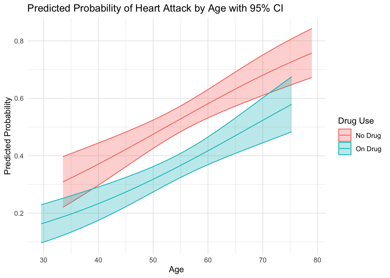
Visualizing Predicted Probabilities
To provide a tangible representation, let’s plot the predicted probabilities of heart attacks by age from our model:
library(ggplot2)data_high_risk$predicted_prob <-predict(model_high_risk, type ="response")predictions <-predict(model_high_risk, type ="response", se.fit =TRUE)data_high_risk$lower_ci <- predictions$fit -1.96* predictions$se.fitdata_high_risk$upper_ci <- predictions$fit +1.96* predictions$se.fitggplot(data_high_risk, aes(x = age, y = predicted_prob, color =as.factor(drug_use))) +geom_ribbon(aes(ymin = lower_ci, ymax = upper_ci, fill =as.factor(drug_use)), alpha =0.3) +geom_line() +labs(title ="Predicted Probability of Heart Attack by Age with 95% CI",y ="Predicted Probability",x ="Age",color ="Drug Use",fill ="Drug Use") +scale_color_discrete(labels =c("No Drug", "On Drug")) +scale_fill_discrete(labels =c("No Drug", "On Drug")) +theme_minimal()
The visual clearly illustrates the beneficial effect of the drug over time. It gives a tangible sense of how the risk of heart attacks evolves with age for both groups and the significant advantage of drug users. This can be especially useful for diagnostic purposes or to demonstrate the results of your model to stakeholders.
Conclusion: A Call to Transition
The era of odds ratios has provided us with valuable insights, but as the field of health research progresses, so should our statistical tools and reporting practices. Marginal effects and predicted probabilities provide clearer, more intuitive insights, pushing us away from the ambiguous realm of odds and into the tangible world of real impact.
After all, the end goal of our research is to provide clear, actionable insights that can be readily applied to improve health outcomes. Let’s choose clarity over tradition, and marginal effects over odds ratios.