Section 7 - Non-linear Models

Author

Jacob Jameson

Note: this section has several different types of models. We cannot cover all of them in 1.25 hours. We will go over a few examples but once you understand how the examples, you should be able to apply the logic to other types models.

This week, we will use the Wage data that is part of the ISLR package

library(ISLR)

Load the Wage data and drop the “Wage” columns, as we did in Section 6

wage_data <- Wage
wage_data <- wage_data[, -10]

To make life easier for later analyses, I will start by sorting the data on age. To do this, I will use a package called dplyr, which has a lot of great tools for data manipulation.

library(dplyr)

The first two functions we will use are: - %>% which means “and then do” - arrange() which sorts the data on the column inside the parentheses

wage_data <- wage_data %>% arrange(age)

We will start by splitting the data into training and test sets

set.seed(222)
train <- sample(1:nrow(wage_data), round(nrow(wage_data) * 0.8))
train <- sort(train)
test <- which(!(seq(nrow(wage_data)) %in% train))

To quickly and easily measure MSEP, write our own function

msep_func <- function(predictions, true_vals) {
  MSEP <- mean((predictions - true_vals)^2)
  return(MSEP)
}

Polynomial Regression

We can start by fitting a polynomial regression using only age

age_poly <- lm(wage ~ poly(age, 4), data = wage_data[train,])

Extract the coefficients from the model

coef(summary(age_poly))

                Estimate Std. Error    t value     Pr(>|t|)
(Intercept)    111.88351  0.8086511 138.358203 0.000000e+00
poly(age, 4)1  394.18926 39.6156514   9.950342 6.942194e-23
poly(age, 4)2 -434.00566 39.6156514 -10.955409 2.748637e-27
poly(age, 4)3  105.56550 39.6156514   2.664742 7.756432e-03
poly(age, 4)4  -90.09776 39.6156514  -2.274297 2.303622e-02

When you use poly(), it returns a matrix of “orthogonal polynomials” so the columns of the matrix are linear combinations of age, age\(^2\), age\(^3\), age\(^4\). Let’s take a look!

head(poly(wage_data$age, 4))

              1          2           3          4
[1,] -0.0386248 0.05590873 -0.07174058 0.08672985
[2,] -0.0386248 0.05590873 -0.07174058 0.08672985
[3,] -0.0386248 0.05590873 -0.07174058 0.08672985
[4,] -0.0386248 0.05590873 -0.07174058 0.08672985
[5,] -0.0386248 0.05590873 -0.07174058 0.08672985
[6,] -0.0386248 0.05590873 -0.07174058 0.08672985

head(wage_data$age)

[1] 18 18 18 18 18 18

If you want it to return the raw powers of age, you can add an argument to the function poly()

head(poly(wage_data$age, 4, raw = TRUE))

      1   2    3      4
[1,] 18 324 5832 104976
[2,] 18 324 5832 104976
[3,] 18 324 5832 104976
[4,] 18 324 5832 104976
[5,] 18 324 5832 104976
[6,] 18 324 5832 104976

Although the two forms give you different numbers, they result in the same predictions, because your model is still a linear combination of the original powers

age_poly_TRUE <- lm(wage ~ poly(age, 4, raw = TRUE), 
                    data = wage_data[train,])

Extract the coefficients from the model

coef(summary(age_poly_TRUE))

                               Estimate   Std. Error   t value     Pr(>|t|)
(Intercept)               -2.085312e+02 6.559430e+01 -3.179106 0.0014961570
poly(age, 4, raw = TRUE)1  2.391179e+01 6.439356e+00  3.713383 0.0002091772
poly(age, 4, raw = TRUE)2 -6.646745e-01 2.257678e-01 -2.944063 0.0032705193
poly(age, 4, raw = TRUE)3  8.403840e-03 3.362741e-03  2.499105 0.0125172334
poly(age, 4, raw = TRUE)4 -4.098605e-05 1.802141e-05 -2.274297 0.0230362203

We can see from the coefficient outputs of the two models that they have different coefficients. We will now check that they make the same predictions.

age_poly_pred <- predict(age_poly, newdata = wage_data[test,])
age_poly_TRUE_pred  <- predict(age_poly_TRUE, newdata = wage_data[test,])

Explore the predictions

head(age_poly_pred)

       5       19       26       32       37       41 
51.23518 58.14597 64.50781 64.50781 64.50781 64.50781

head(age_poly_TRUE_pred)

       5       19       26       32       37       41 
51.23518 58.14597 64.50781 64.50781 64.50781 64.50781

Calculate and print the MSEP

print(msep_func(age_poly_pred, wage_data[test, "wage"]))

[1] 1689.522

cbind() is a function that joins columns together by binding them next to each other. There is also a function rbind() that joins by binding new rows to the bottom of old ones. Let’s try using cbind() to look at both sets of predictions at the same time:

pred_comparison <- cbind(age_poly_pred, age_poly_TRUE_pred)

The column names default to the variable names, but ifwe want to change them, we can use the colnames() function

colnames(pred_comparison) <- c("pred1", "pred2")

We can then generate a variable that flags any instances where the predictions do not line up. To do this, I will introduce you another function in dplyr: mutate() which means create a new variable

pred_comparison <- pred_comparison %>% 
  mutate(check_same = as.numeric(pred1 == pred2))

Error in UseMethod("mutate") : no applicable method for 'mutate' applied to an object of class "c('matrix', 'array', 'double', 'numeric')"

The previous line errored because pred_comparison is a matrix and dplyr was designed to work on data frames.

Make pred_comparison a data frame

pred_comparison <- data.frame(pred_comparison)

Now try running the code:

pred_comparison <- pred_comparison %>%
  mutate(check_same = as.numeric(pred1 == pred2))

View the results

View(pred_comparison)

Regression Splines

Splines

We’re going to start by making an age grid, so that we test our predictions on a grid of evenly spaced ages so that you capture the functional form well.

A quick aside, na.rm = TRUE means exlucde missing observations. Then we are going to run a spline with knots at ages 25, 40, and 60.

library(splines)

Create the age grids

age_grid <- seq(from = min(wage_data$age, na.rm = TRUE),
                to = max(wage_data$age, na.rm = TRUE))

Now we use a basis function

spline_age <- lm(wage ~ bs(age, knots = c(25, 40, 60)), 
                 data = wage_data[train,])

?bs # to check what the basis function does

Get the predictions at the grid points we defined earlier

spline_age_grid_pred  <- predict(spline_age, 
                                 newdata = list(age = age_grid), 
                                 se = TRUE)

Plot age on the x-axis and wage on the y-axis for the test data. Then add the predictions and the confidence intervals

plot(wage_data[test, "age"], wage_data[test, "wage"],
cex = 0.5, col = "darkgrey",
xlab = "age", ylab = "wage")
lines(age_grid, spline_age_grid_pred$fit, lwd = 2)
lines(age_grid, spline_age_grid_pred$fit + 
        2 * spline_age_grid_pred$se, lty ="dashed")
lines(age_grid, spline_age_grid_pred$fit - 
        2 * spline_age_grid_pred$se, lty ="dashed")

Natural Splines

If we instead wanted to fit a natural spline, we use ns() instead of knots, we can specify degrees of freedom. In this case we are going to use 4 degrees of freedom.

ns_age_poly <- lm(wage ~ ns(age, df = 4), data = wage_data[train,])
ns_age_grid_poly_pred <- predict(ns_age_poly,
                                 newdata = list(age = age_grid),
                                 se = TRUE)

plot(wage_data[test, "age"], wage_data[test, "wage"], 
     cex = 0.5, col = "darkgrey",
     xlab = "age", ylab = "wage")
lines(age_grid, ns_age_grid_poly_pred$fit, lwd = 2)
lines(age_grid, ns_age_grid_poly_pred$fit + 
        2 * ns_age_grid_poly_pred$se, lty = "dashed")
lines(age_grid, ns_age_grid_poly_pred$fit - 
        2 * ns_age_grid_poly_pred$se, lty = "dashed")

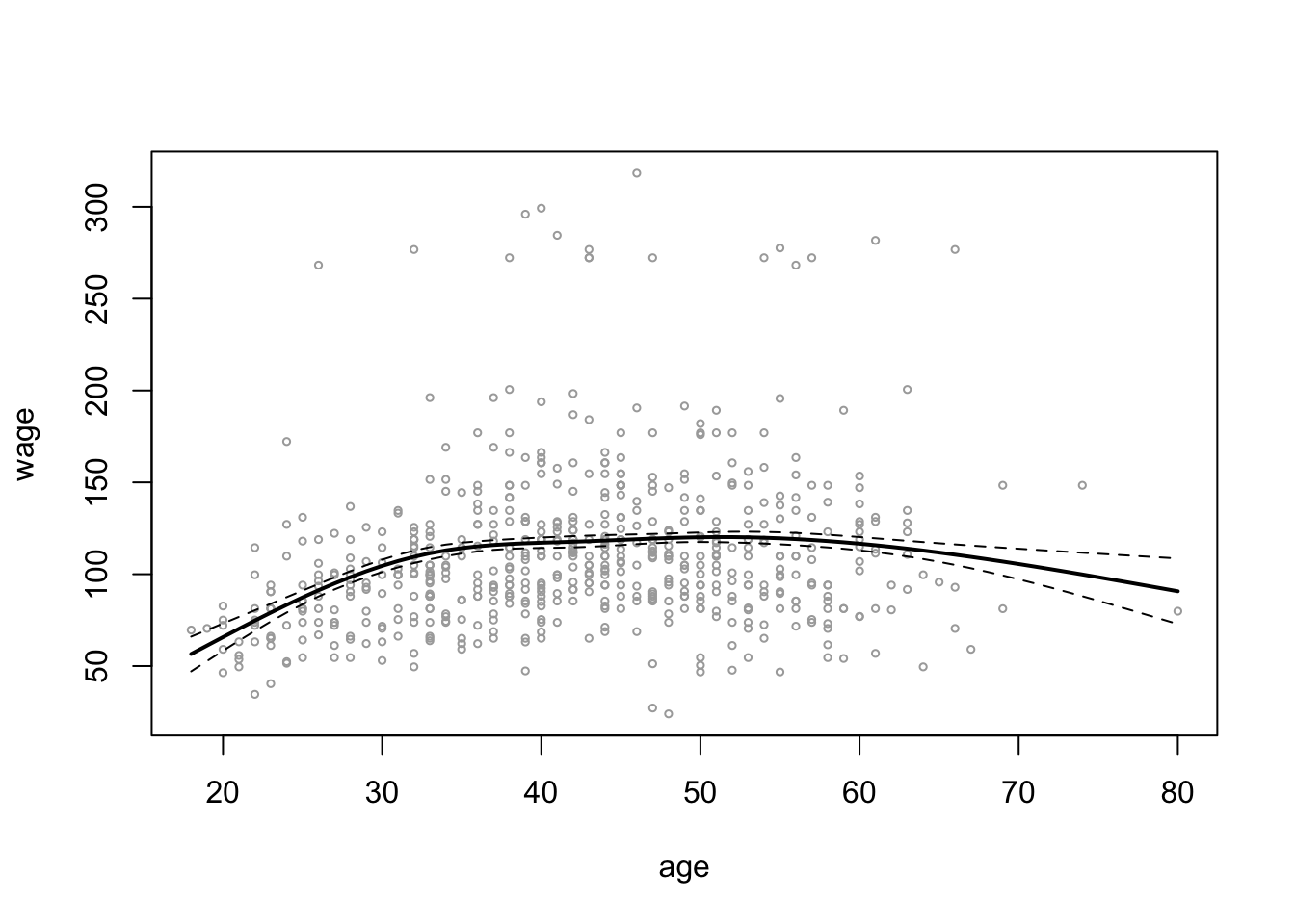
Smoothing Splines

To fit a smoothing spline, we use smooth.spline(). We can specify our own df

smooth_age <- smooth.spline(wage_data[train,"age"], 
                            wage_data[train, "wage"], 
                            df = 16)

Or we can use cross Validation to get optimal df and penalty

smoothCV_age <- smooth.spline(wage_data[train, "age"], 
                              wage_data[train, "wage"], 
                              cv = TRUE) # specify we want to use CV
smoothCV_age$df

[1] 6.786486

Plot the results as before

plot(wage_data[test, "age"], wage_data[test, "wage"],
     cex =.5, col = "darkgrey",
     xlab = "age", ylab = "wage")
title(" Smoothing Spline ")
lines(smooth_age, col ="red", lwd = 2)
lines(smoothCV_age, col ="blue", lwd =2)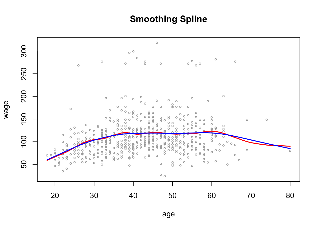

Local Regression

Local Regression use loess()

Note: span = 0.2 makes neighborhoods with 20% of observations. Span = 0.5 creates neighborhoods with 50% of observations. So the larger the span, the smoother the fit

# plot age and wage and add geom_smooth
library(ggplot2)
ggplot(wage_data[test,], aes(x = age, y = wage, color = education)) +
  geom_point(alpha = 0.5) +
  geom_smooth(method = "loess", span = 0.2) +
  geom_smooth(method = "loess", span = 0.5)

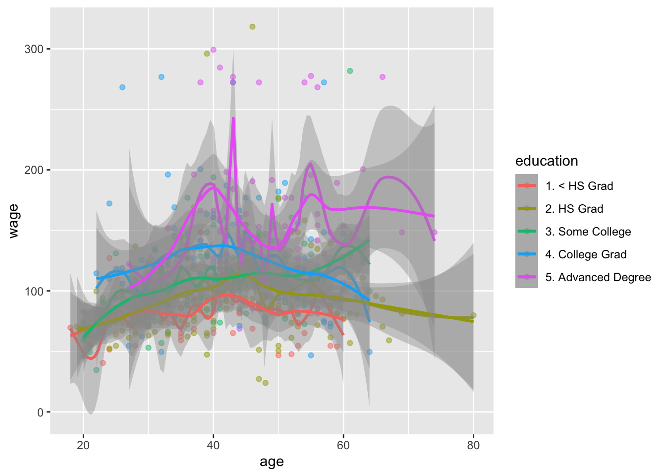
local2_age <- loess(wage ~ age, span = 0.2, data = wage_data)
local5_age <- loess(wage ~ age, span = 0.5, data = wage_data)

Get the predictions

pred_local2_age <- predict(local2_age, newdata = data.frame(age = age_grid))
pred_local5_age <- predict(local5_age, newdata = data.frame(age = age_grid))

Plot the results

plot(wage_data[test, "age"], wage_data[test, "wage"],
     cex =.5, col = "darkgrey",
     xlab = "age", ylab = "wage")
lines(age_grid, pred_local2_age, col = "red", lwd = 2)
lines(age_grid, pred_local5_age, col = "blue", lwd = 2)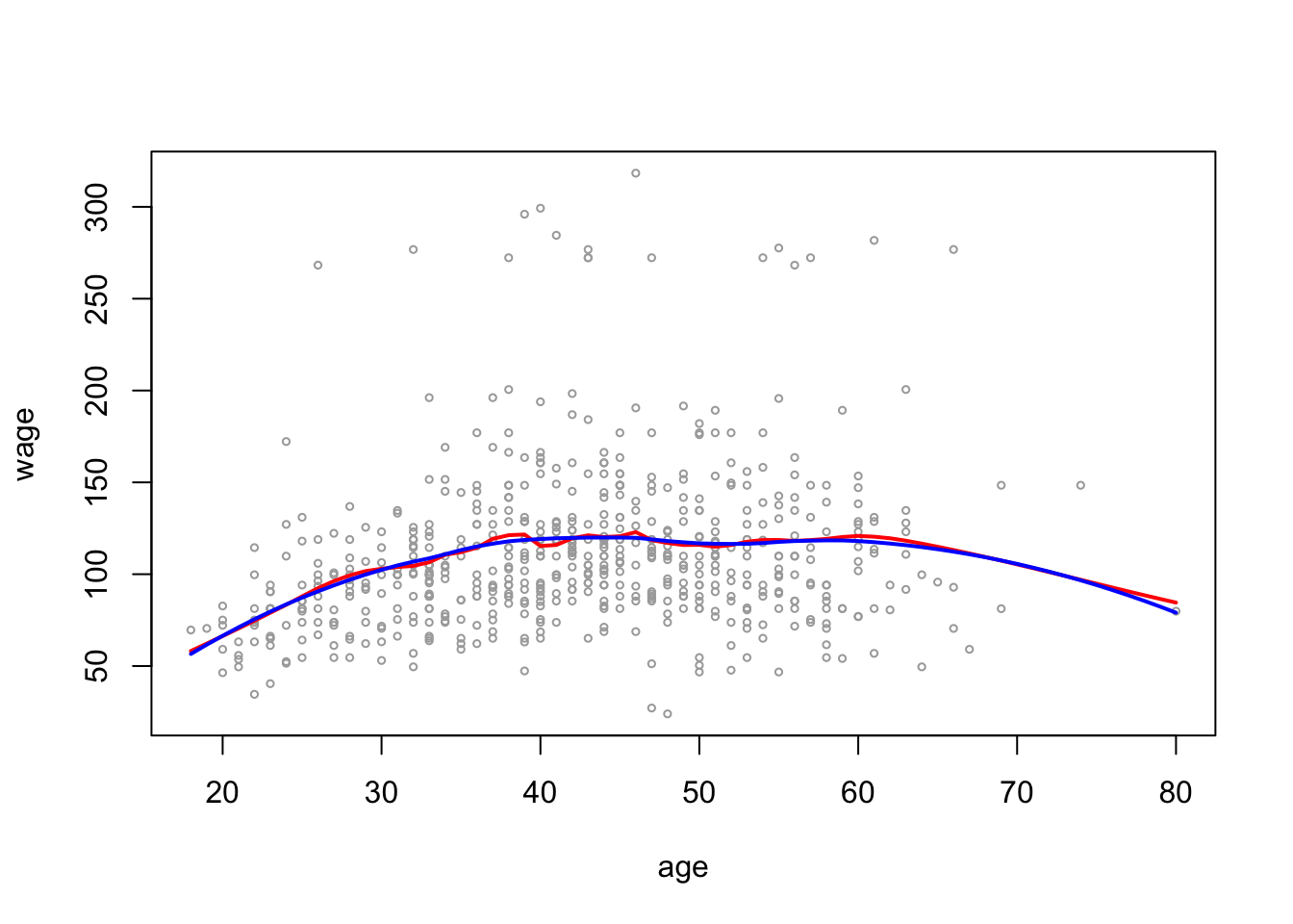

GAMs

Generalized Additive Models (GAMs)

Start with using natural spline functions of year and age and treating education as a qualitative variable does not require any special packages

Example 1: GAMs with splines

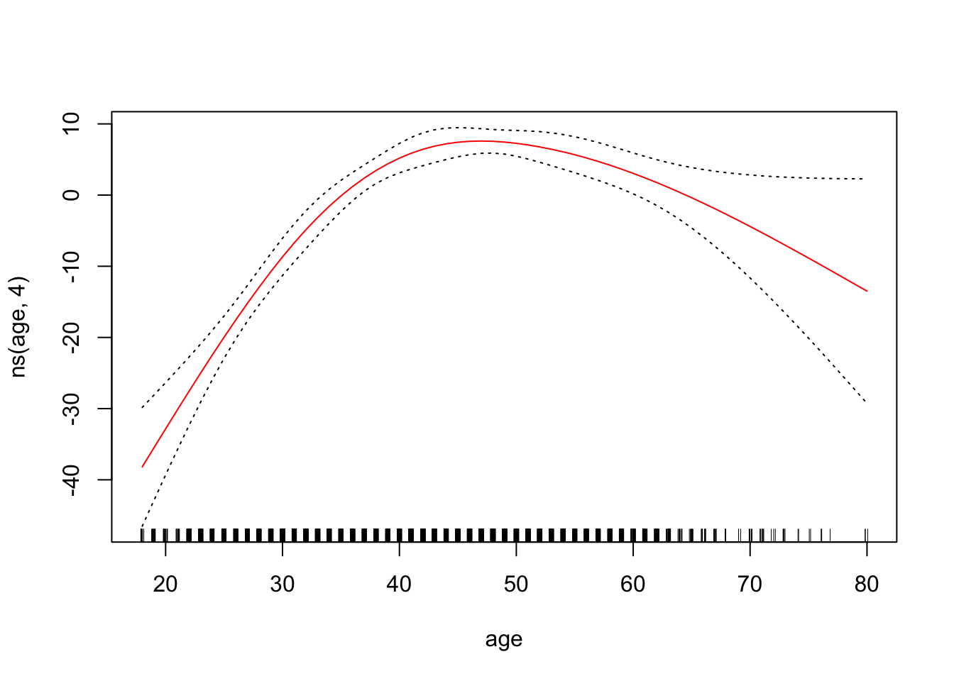
gam_yae <- lm(wage ~ ns(year, 4) + ns(age, 4) + education, 
              data = wage_data[train,])

Example 2: GAMs with smoothing splines

library(gam)

In the gam library s() indicates that we want to use a smoothing spline

gam_smooth <- gam(wage ~ s(year, 4, spar = 0.5) + s(age, 5) + education,
                  data = wage_data[train,])

Plot the model results

par(mfrow = c(1, 3))
plot(gam_smooth, se = TRUE, col ="blue ")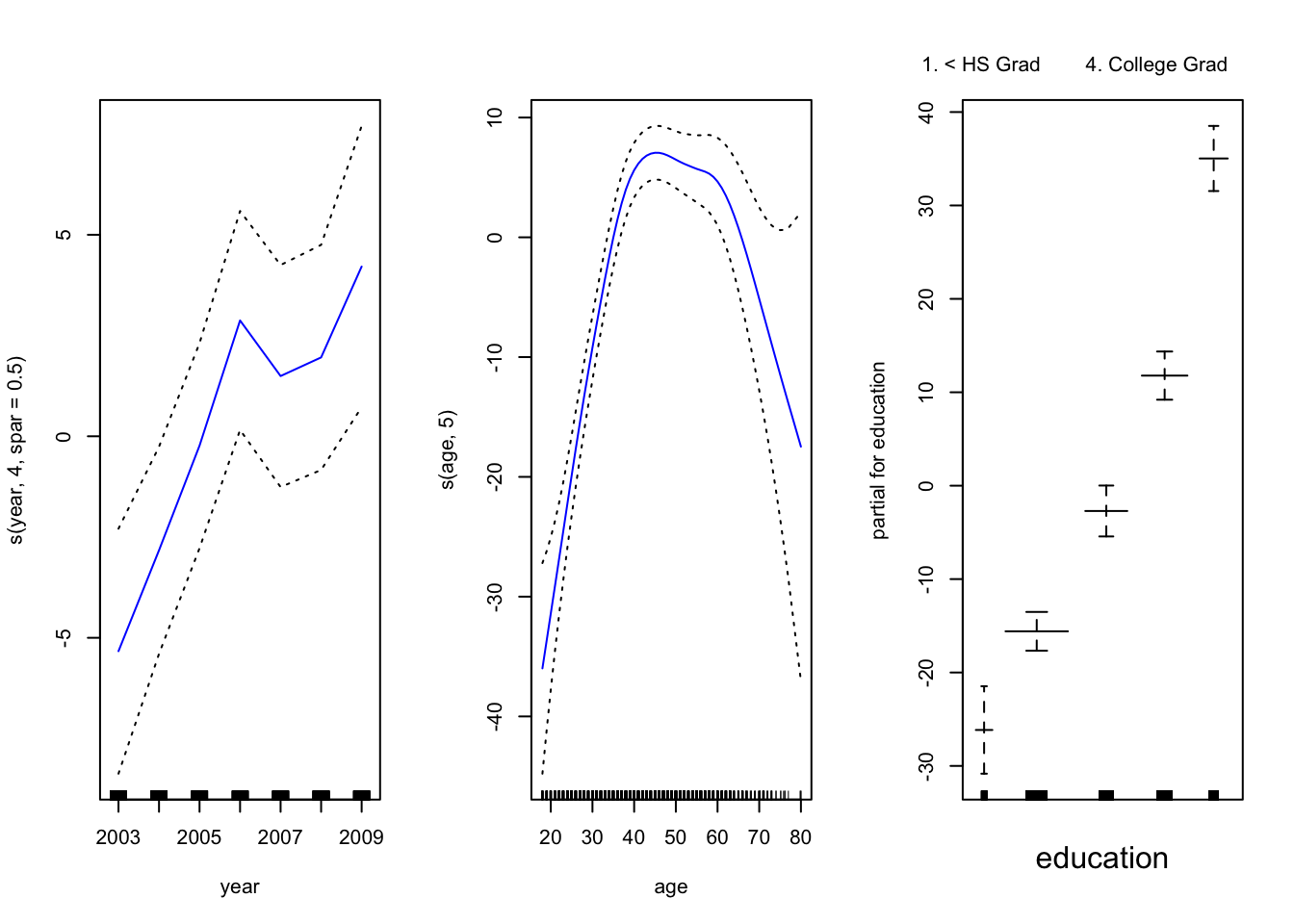

To plot the GAM we created just using lm(), we can use plot.Gam()

plot.Gam(gam_yae, se = TRUE, col = "red") # Note the capitalization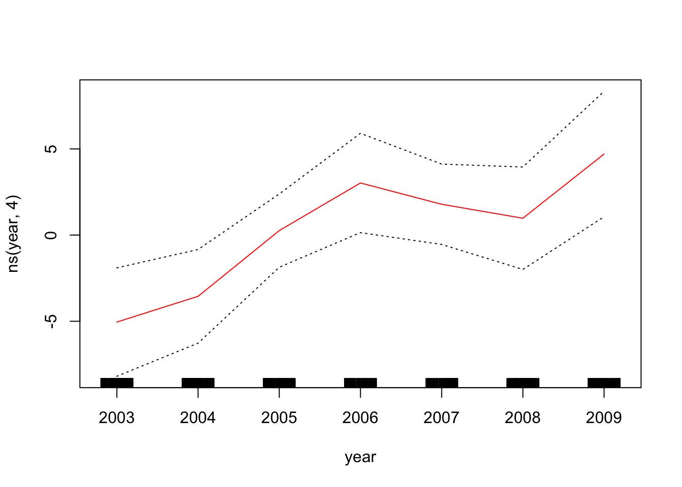

Make predictions

gam_yae_pred <- predict(gam_yae, newdata = wage_data[test,])
gam_smooth_pred <- predict(gam_smooth, newdata = wage_data[test,])

Print out the MSEP for these two GAMs using the function we created at the start of class

print(msep_func(gam_yae_pred, wage_data[test, "wage"]))

[1] 1304.807

print(msep_func(gam_smooth_pred, wage_data[test, "wage"]))

[1] 1300.582

Example 3: GAMs with local regression

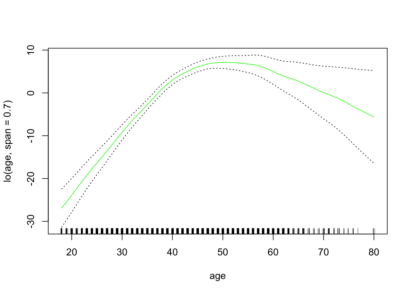
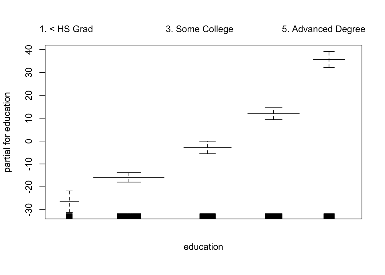
To use local regression in GAMs, use lo()

gam_lo <- gam(wage ~ s(year, df = 4) + lo(age, span = 0.7) + education, 
              data = wage_data[train,])

Plot the results

plot.Gam(gam_lo, se = TRUE, col = "green")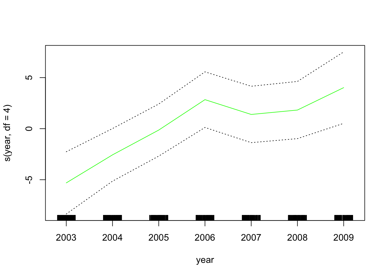

If you want to do a local regression in two variables:

gam_2lo <- gam(wage ~ lo(year, age, span =0.5) + education,
               data = wage_data[train,])

Warning in lo.wam(x, z, wz, fit$smooth, which, fit$smooth.frame, bf.maxit, :
liv too small.  (Discovered by lowesd)

Warning in lo.wam(x, z, wz, fit$smooth, which, fit$smooth.frame, bf.maxit, : lv
too small.  (Discovered by lowesd)

Warning in lo.wam(x, z, wz, fit$smooth, which, fit$smooth.frame, bf.maxit, :
liv too small.  (Discovered by lowesd)

Warning in lo.wam(x, z, wz, fit$smooth, which, fit$smooth.frame, bf.maxit, : lv
too small.  (Discovered by lowesd)

?s

Help on topic 's' was found in the following packages:

  Package               Library
  gam                   /opt/homebrew/Cellar/r/4.4.2_2/lib/R/library
  mgcv                  /opt/homebrew/Cellar/r/4.4.2_2/lib/R/library


Using the first match ...