library(ISLR)
insurance_data <- CaravanSection 6 - Regularization and Dimension Reduction
Notes
Note that the material in these notes draws on past TF’s notes (Ibou Dieye, Laura Morris, Emily Mower, Amy Wickett), and the more thorough treatment of these topics in Introduction to Statistical Learning by Gareth James, Daniela Witten, Trevor Hastie and Robert Tibshirani.
The goal of this session is to review concepts related to regularization methods (LASSO and Ridge Regression) and dimension reduction techniques (PCA and PLS).
LASSO and Ridge Regression
Concept
Least Absolute Shrinkage and Selection Operator (LASSO) and Ridge Regression both fall under a broader class of models called shrinkage models. Shrinkage models regularize or penalize coefficient estimates, which means that they shrink the coefficients toward zero. Shrinking the coefficient estimates can reduce their variance, so these methods are particularly useful for models where we are concerned about high variance (i.e. over-fitting), such as models with a large number of predictors relative to the number of observations.
Both LASSO and Ridge regression operate by adding a penalty to the normal OLS (Ordinary Least Squares) minimization problem. These penalties can be thought of as a budget, and sometimes the minimization problem is explicitly formulated as minimizing the Residual Sum of Squares (RSS) subject to a budget constraint. The idea of the budget is if you have a small budget, you can only afford a little “total” \(\beta\), where the definition of “total” \(\beta\) varies between LASSO and Ridge, but as your budget increases, you get closer and closer to the OLS \(\beta\)s.
LASSO and Ridge regression differ in exactly how they penalize the coefficients. In particular, LASSO penalizes the coefficients using an \(L_1\) penalty:
\[ \sum_{i=1}^n \left( y_i - \beta_0 - \sum_{j=1}^p \beta_j x_{ij} \right)^2 + \lambda \sum_{j=1}^p |\beta_j| = RSS + \lambda \sum_{j=1}^p |\beta_j| \]
Ridge regression penalizes the coefficients using an \(L_2\) penalty:
\[ \sum_{i=1}^n \left( y_i - \beta_0 - \sum_{j=1}^p \beta_j x_{ij} \right)^2 + \lambda \sum_{j=1}^p \beta_j^2 = RSS + \lambda \sum_{j=1}^p \beta_j^2 \] You may notice that both the LASSO and Ridge Regression minimization problems feature a parameter \(\lambda\). This is a tuning parameter that dictates how much we will penalize the “total” coefficients. Tuning parameters appear in many models and get their name from the fact that we tune (adjust / choose) them in order to improve our model’s performance.
Since LASSO and Ridge Regression are used when we are concerned about variance (over-fitting), it should come as no surprise that increasing \(\lambda\) decreases variance. It can be helpful to contextualize the \(\lambda\) size by realizing that \(\lambda=0\) is OLS and \(\lambda =\infty\) results in only \(\beta_0\) being assigned a non-zero value.
As we increase \(\lambda\) from zero, we decrease variance but increase bias (the classic bias-variance tradeoff). To determine the best \(\lambda\) (e.g. the \(\lambda\) that will lead to the best out of sample predictive performance), it is common to use cross validation. A good function in R that trains LASSO and Ridge Regression models and uses cross-validation to select a good \(\lambda\) is cv.glmnet(), which is part of the glmnet package.
Key difference between LASSO and Ridge
As noted above, both LASSO and Ridge regression shrink the coefficients toward zero. However, the penalty in Ridge (\(\lambda \beta_j^2\)) will not set any of coefficients exactly to zero (unless \(\lambda =\infty\)). Increasing the value of \(\lambda\) will tend to reduce the magnitudes of the coefficients (which helps reduce variance), but will not result in exclusion of any of the variables. While this may not impact prediction accuracy, it can create a challenge in model interpretation in settings where the number of features is large. This is an obvious disadvantage.
On the other hand, the \(L_1\) penalty of LASSO forces some of the coefficient estimates to be exactly equal to zero when the tuning parameter \(\lambda\) is sufficiently large. Therefore, LASSO performs variable selection, much like best subset selection.
Implementation and Considerations
LASSO and Ridge Regression are useful models to use when dealing with a large number of predictors \(p\) relative to the number of observations \(n\). It is good to standardize your features so that coefficients are not selected because of their scale rather than their relative importance.
For example, suppose you were predicting salary, and suppose you had a standardized test score that was highly predictive of salary and you also had parents’ income, which was only somewhat predictive of salary. Since standardized test scores are measured on a much smaller scale than the outcome and than parents’ income, we would expect the coefficient on test scores to be large relative to the coefficient on parents’ income. This means it would likely be shrunk by adding the penalty, even though it reflects a strong predictive relationship.
Interpreting Coefficients
Coefficients produced by LASSO and Ridge Regression should not be interpreted causally. These methods are used for prediction, and as such, our focus is on \(\hat{y}\). This is in contrast to an inference problem, where we would be interested in \(\hat{\beta}\).
The intuition behind why we cannot interpret the coefficients causally is similar to the intuition underlying Omitted Variables Bias (OVB). In OVB, we said that if two variables \(X_1\) and \(X_2\) were correlated with each other and with the outcome \(Y\), then the coefficient on \(X_1\) in a regression of \(Y\) on \(X_1\) would differ from the coefficient on \(X_1\) in a regression where \(X_2\) was also included. This is because since \(X_1\) and \(X_2\) are correlated, when we omit \(X_2\), the coefficient on \(X_1\) picks up the effect of \(X_1\) on \(Y\) as well as some of the effect of \(X_2\) on \(Y\).
Principal Components Analysis and Regression
Principal Components Analysis
Principal Components Analysis is a method of unsupervised learning. We have not yet covered unsupervised learning, though we will in the second half of the semester. The important thing to know at this point about unsupervised learning is that unsupervised learning methods do not use labels \(Y\).
Principal Components Analysis (PCA), therefore, does not use \(Y\) in determining the principal components. Instead, the principal components are determined solely by looking at the predictors \(X_1\),…,\(X_p\). Each principal component is a weighted sum of the original predictors \(X_1\),…,\(X_p\). For clarity of notation, we will use \(Z\) to represent principal components and \(X\) to represent predictors.
Principal components are created in an ordered way. The order can be described as follows: If you had to project all of the data onto only one line, the first principal component defines the line that would lead to points being as spread out as possible (e.g. having highest variance). If you had to project all of the data onto only one plane, the plane defined by the first two principal components (which are orthogonal by definition) would be the plane where the points were as spread out as possible (e.g. highest possible variance).
Since variance is greatly affected by measurement scale, it is common practice and a good idea to scale your variables, so that results are not driven by the scale on which the variables were measured.
When estimating principal components, you will estimate \(p\) components, where \(p\) is the number of predictors \(X\). However, you usually only pay attention to / use the first few components, since the last few components capture very little variance. Note that you can exactly recover your original data when using all \(p\) components.
Principal Components Regression
Principal Components Regression (PCR) regresses the outcome \(Y\) on the principal components \(Z_1\),…,\(Z_M\), where \(M<p\) and \(p\) is the number of predictors \(X_1\),…,\(X_p\).
Note that the principal components \(Z_1\),…,\(Z_M\) were defined by looking only at \(X_1\),…,\(X_p\) and not at \(Y\). Putting the principal components into a regression is the first time we are introducing any interaction between the principal components and the outcome \(Y\).
The main idea of Principal Components Regression is that hopefully only a few components explain most of the variance in the predictors overall and as is relevant to the relationship between the predictors and the response. In other words, when we use PCR, we assume that the directions in which \(X\) shows the most variance are also the directions most associated with \(Y\). When this assumption is true, we are able to use \(M<<p\) (e.g. \(M\) much smaller than \(p\)) parameters while still getting similar in-sample performance and hopefully better out-of-sample performance (due to not overfitting) to a regression of \(Y\) on all \(p\) predictors. Although the assumption is not guaranteed to be true, it is often a good enough approximation to give good results.
PCA is one example of dimensionality reduction, because it reduces the dimension of the problem from \(p\) to \(M\). Note, though, that dimensionality reduction is different from feature selection. We are still using all features; we have just aggregated them into principal components.
The exact number \(M\) of principal components to use in PCR (the regression of \(Y\) on the principal components) is usually determined by cross-validation.
Implementation and Considerations
When using PCR, there are a few things to pay attention to. First, be sure to standardize variables or else the first few principal components will favor features measured on larger scales. Second, the number of principal components to use in PCR is determined using cross-validation. If the number is high and close to the number of features in your data, the assumption that the directions in which the predictors vary most are also the directions that explain the relationship between the predictors and response is false. In such a case, other methods, such as ridge and lasso, are likely to perform better.
Partial Least Squares
Partial Least Squares is a supervised alternative to PCR. Recall that for PCR, the principal components \(Z_1,...,Z_M\) were formed from the original features \(X_1,...,X_p\) without looking at \(Y\) (unsupervised).
Partial Least Squares (PLS) also generates a new set of features \(Z_1,...,Z_M\) but it uses the correlation between the predictors \(X_1,...,X_p\) and the outcome \(Y\) to determine the weights on \(X_1,...,X_p\) for each \(Z_1,...,Z_M\). In this way, PLS attempts to find directions that explain both the response and the predictors.
The first feature \(Z_1\) is determined by weighting \(X_1,...,X_p\) proportional to each feature’s correlation with \(Y\). It then residualizes the predictors \(X_1,...,X_p\) by regressing them on \(Z_1\) and repeats the weighting procedure using the orthogonalized predictors. The process then repeats until we have \(M\) components, where \(M\) is determined by cross validation.
Implementation and Considerations
Just as with PCR, it’s best practice to scale the predictors before running PLS.
Comparison with PCR
PLS directly uses \(Y\) in generating the features \(Z_1,...,Z_M\). It then regresses \(Y\) on these features. Therefore, PLS uses \(Y\) twice in the process of estimating the model.
In contrast, PCR only looks at the outcome \(Y\) when estimating the final regression. The components are estimated without ``peeking’’ at \(Y\).
Because \(Y\) is used twice in PLS and only once in PCR, in practice PLS exhibits lower bias (e.g. is better able to fit the training data) but higher variance (e.g. is more sensitive to the exact training data). Therefore, the two methods generally have similar out-of-sample predictive power in practice.
Coding
LASSO and Ridge Regression
We will use the Caravan data set that is included in the package ISLR. This data set contains information on people offered Caravan insurance.
Let’s learn a little more about the data
?CaravanLet’s try to predict CARAVAN. Note: although this is a binary variable, ridge and lasso are regression algorithms – regression can often give you a good sense of the ordinal distribution of likelihood that the outcome will be 1 even if the resulting value cannot be viewed as a probability). When you run lasso and ridge, you will need to provide a penalty parameter. Since we don’t know which penalty parameter is best, we will use a built in cross-validation function to find the best penalty parameter (lambda) in the package glmnet
library(glmnet)Loading required package: MatrixLoaded glmnet 4.1-8?cv.glmnetWe will start by using the function’s built-in sequence of lambdas and glmnet standardization
set.seed(222) # Important for replicability
lasso_ins <- cv.glmnet(x = as.matrix(insurance_data[, 1:85]), # the features
                       y = as.numeric(insurance_data[, 86]), # the outcome
                       standardize = TRUE, # Why do we do this?
                       alpha = 1) # Corresponds to LASSO
We can see which lambda sequence was used
print(lasso_ins$lambda) [1] 3.577561e-02 3.259740e-02 2.970154e-02 2.706294e-02 2.465874e-02
[6] 2.246812e-02 2.047212e-02 1.865343e-02 1.699631e-02 1.548641e-02
[11] 1.411064e-02 1.285709e-02 1.171490e-02 1.067418e-02 9.725915e-03
[16] 8.861891e-03 8.074625e-03 7.357298e-03 6.703696e-03 6.108158e-03
[21] 5.565526e-03 5.071100e-03 4.620597e-03 4.210116e-03 3.836101e-03
[26] 3.495312e-03 3.184799e-03 2.901870e-03 2.644076e-03 2.409183e-03
[31] 2.195158e-03 2.000146e-03 1.822459e-03 1.660557e-03 1.513037e-03
[36] 1.378623e-03 1.256150e-03 1.144557e-03 1.042878e-03 9.502315e-04
[41] 8.658156e-04 7.888989e-04 7.188153e-04 6.549577e-04 5.967731e-04
[46] 5.437574e-04 4.954515e-04 4.514370e-04 4.113325e-04 3.747909e-04
[51] 3.414955e-04 3.111580e-04 2.835156e-04 2.583288e-04 2.353796e-04
[56] 2.144691e-04 1.954163e-04 1.780560e-04 1.622380e-04 1.478253e-04
[61] 1.346929e-04 1.227271e-04 1.118244e-04 1.018902e-04 9.283857e-05
[66] 8.459104e-05 7.707621e-05 7.022897e-05 6.399002e-05 5.830533e-05
[71] 5.312564e-05 4.840611e-05 4.410584e-05 4.018760e-05 3.661744e-05
[76] 3.336445e-05 3.040045e-05 2.769975e-05 2.523898e-05 2.299682e-05
[81] 2.095385e-05 1.909237e-05 1.739625e-05 1.585082e-05 1.444267e-05
[86] 1.315963e-05 1.199056e-05 1.092535e-05 9.954775e-06 9.070420e-06
[91] 8.264629e-06 7.530422e-06 6.861440e-06 6.251889e-06 5.696488e-06
[96] 5.190428e-06 4.729325e-06 4.309185e-06 3.926368e-06 3.577561e-06Let’s find the lambda that does the best as far as CV error goes
print(lasso_ins$lambda.min)[1] 0.006703696You can plot the model results
plot(lasso_ins)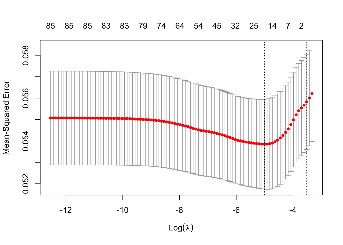
You can also plot the CV-relevant outputs
LassoCV <- lasso_ins$glmnet.fit

plot(LassoCV, label = TRUE, xvar = "lambda")

abline(
  v = log(c(lasso_ins$lambda.min, lasso_ins$lambda.1se))
  ) # Adds lines to mark the two key lambda values
You can see the coefficients corresponding to the two key lambda values using the predict function
predict(lasso_ins, type = "coefficients",
        s = c(lasso_ins$lambda.min, lasso_ins$lambda.1se))
86 x 2 sparse Matrix of class "dgCMatrix"
s1 s2
(Intercept) 0.9896239538 1.053595130
MOSTYPE . .
MAANTHUI . .
MGEMOMV . .
MGEMLEEF . .
MOSHOOFD . .
MGODRK . .
MGODPR . .
MGODOV . .
MGODGE . .
MRELGE 0.0018180263 .
MRELSA . .
MRELOV . .
MFALLEEN . .
MFGEKIND . .
MFWEKIND . .
MOPLHOOG 0.0022611683 .
MOPLMIDD . .
MOPLLAAG -0.0024753875 .
MBERHOOG . .
MBERZELF . .
MBERBOER -0.0030373898 .
MBERMIDD . .
MBERARBG . .
MBERARBO . .
MSKA . .
MSKB1 . .
MSKB2 . .
MSKC . .
MSKD . .
MHHUUR -0.0007565131 .
MHKOOP . .
MAUT1 0.0013643467 .
MAUT2 . .
MAUT0 . .
MZFONDS . .
MZPART . .
MINKM30 . .
MINK3045 . .
MINK4575 . .
MINK7512 . .
MINK123M . .
MINKGEM 0.0028225067 .
MKOOPKLA 0.0025557889 .
PWAPART 0.0076586029 .
PWABEDR . .
PWALAND -0.0008184860 .
PPERSAUT 0.0087316235 0.002079863
PBESAUT . .
PMOTSCO . .
PVRAAUT . .
PAANHANG . .
PTRACTOR . .
PWERKT . .
PBROM . .
PLEVEN . .
PPERSONG . .
PGEZONG . .
PWAOREG 0.0010472132 .
PBRAND 0.0042630439 .
PZEILPL . .
PPLEZIER . .
PFIETS . .
PINBOED . .
PBYSTAND . .
AWAPART . .
AWABEDR . .
AWALAND . .
APERSAUT 0.0006293082 .
ABESAUT . .
AMOTSCO . .
AVRAAUT . .
AAANHANG . .
ATRACTOR . .
AWERKT . .
ABROM . .
ALEVEN . .
APERSONG . .
AGEZONG . .
AWAOREG . .
ABRAND . .
AZEILPL . .
APLEZIER 0.2083116609 .
AFIETS 0.0076146528 .
AINBOED . .
ABYSTAND 0.0361586998 . Questions you should be able to answer :
- Which lambda in the sequence had the lowest CV error?
lasso_ins$lambda.min[1] 0.006703696- What is the CV error of the “best” lambda?
lasso_ins$cvm[lasso_ins$lambda == lasso_ins$lambda.min][1] 0.05384566- What is the standard deviation of the CV error for the “best” lambda?
lasso_ins$cvsd[lasso_ins$lambda == lasso_ins$lambda.min][1] 0.002099205- What is the largest lambda whose CV error was within 1 standard error of the lowest CV error?
lasso_ins$lambda.1se[1] 0.02970154When you do ridge regression, the code is almost exactly the same as for lasso in R. You just need to change the alpha parameter from 1 to 0. I’ll leave this to you as an exercise.
Principal Components Analysis (PCA) and Partial Least Squares (PLS)
We will use the Wage data set that is included in the package ISLR. This data set contains information on people’s wages.
wage_data <- WageLet’s learn a little more about the data
summary(wage_data)The data set contains 3000 observations on 11 variables. The variables are:
str(wage_data)'data.frame': 3000 obs. of 11 variables:
$ year : int 2006 2004 2003 2003 2005 2008 2009 2008 2006 2004 ...
$ age : int 18 24 45 43 50 54 44 30 41 52 ...
$ maritl : Factor w/ 5 levels "1. Never Married",..: 1 1 2 2 4 2 2 1 1 2 ...
$ race : Factor w/ 4 levels "1. White","2. Black",..: 1 1 1 3 1 1 4 3 2 1 ...
$ education : Factor w/ 5 levels "1. < HS Grad",..: 1 4 3 4 2 4 3 3 3 2 ...
$ region : Factor w/ 9 levels "1. New England",..: 2 2 2 2 2 2 2 2 2 2 ...
$ jobclass : Factor w/ 2 levels "1. Industrial",..: 1 2 1 2 2 2 1 2 2 2 ...
$ health : Factor w/ 2 levels "1. <=Good","2. >=Very Good": 1 2 1 2 1 2 2 1 2 2 ...
$ health_ins: Factor w/ 2 levels "1. Yes","2. No": 2 2 1 1 1 1 1 1 1 1 ...
$ logwage : num 4.32 4.26 4.88 5.04 4.32 ...
$ wage : num 75 70.5 131 154.7 75 ...To the view the levels of a particular factor variable, we can use:
levels(wage_data$maritl)[1] "1. Never Married" "2. Married" "3. Widowed" "4. Divorced"
[5] "5. Separated" levels(wage_data$region)[1] "1. New England" "2. Middle Atlantic" "3. East North Central"
[4] "4. West North Central" "5. South Atlantic" "6. East South Central"
[7] "7. West South Central" "8. Mountain" "9. Pacific" Notice there is a variable called “wage” and a variable called “logwage”. We just need one of these two. Let’s drop “wage”.
wage_data <- wage_data[, -11]Looking at the data, we see there are integer, factor, and numeric variable types. Let’s convert everything to numeric variables, which includes converting factor variables to a series of indicators.
for(i in 10:1){
  if(is.factor(wage_data[, i])){
    for(j in unique(wage_data[, i])){
      new_col <- paste(colnames(wage_data)[i], j, sep = "_")
      wage_data[, new_col] <- as.numeric(wage_data[, i] == j)
    }
    wage_data <- wage_data[, -i]
  } else if(typeof(wage_data[, i]) == "integer") {
    wage_data[, i] <- as.numeric(as.character(wage_data[, i]))
  }
}
Check your code worked
#View(wage_data)
summary(wage_data)
year age logwage health_ins_2. No
Min. :2003 Min. :18.00 Min. :3.000 Min. :0.0000
1st Qu.:2004 1st Qu.:33.75 1st Qu.:4.447 1st Qu.:0.0000
Median :2006 Median :42.00 Median :4.653 Median :0.0000
Mean :2006 Mean :42.41 Mean :4.654 Mean :0.3057
3rd Qu.:2008 3rd Qu.:51.00 3rd Qu.:4.857 3rd Qu.:1.0000
Max. :2009 Max. :80.00 Max. :5.763 Max. :1.0000
health_ins_1. Yes health_1. <=Good health_2. >=Very Good
Min. :0.0000 Min. :0.000 Min. :0.000
1st Qu.:0.0000 1st Qu.:0.000 1st Qu.:0.000
Median :1.0000 Median :0.000 Median :1.000
Mean :0.6943 Mean :0.286 Mean :0.714
3rd Qu.:1.0000 3rd Qu.:1.000 3rd Qu.:1.000
Max. :1.0000 Max. :1.000 Max. :1.000
jobclass_1. Industrial jobclass_2. Information region_2. Middle Atlantic
Min. :0.0000 Min. :0.0000 Min. :1
1st Qu.:0.0000 1st Qu.:0.0000 1st Qu.:1
Median :1.0000 Median :0.0000 Median :1
Mean :0.5147 Mean :0.4853 Mean :1
3rd Qu.:1.0000 3rd Qu.:1.0000 3rd Qu.:1
Max. :1.0000 Max. :1.0000 Max. :1
education_1. < HS Grad education_4. College Grad education_3. Some College
Min. :0.00000 Min. :0.0000 Min. :0.0000
1st Qu.:0.00000 1st Qu.:0.0000 1st Qu.:0.0000
Median :0.00000 Median :0.0000 Median :0.0000
Mean :0.08933 Mean :0.2283 Mean :0.2167
3rd Qu.:0.00000 3rd Qu.:0.0000 3rd Qu.:0.0000
Max. :1.00000 Max. :1.0000 Max. :1.0000
education_2. HS Grad education_5. Advanced Degree race_1. White
Min. :0.0000 Min. :0.000 Min. :0.0000
1st Qu.:0.0000 1st Qu.:0.000 1st Qu.:1.0000
Median :0.0000 Median :0.000 Median :1.0000
Mean :0.3237 Mean :0.142 Mean :0.8267
3rd Qu.:1.0000 3rd Qu.:0.000 3rd Qu.:1.0000
Max. :1.0000 Max. :1.000 Max. :1.0000
race_3. Asian race_4. Other race_2. Black maritl_1. Never Married
Min. :0.00000 Min. :0.00000 Min. :0.00000 Min. :0.000
1st Qu.:0.00000 1st Qu.:0.00000 1st Qu.:0.00000 1st Qu.:0.000
Median :0.00000 Median :0.00000 Median :0.00000 Median :0.000
Mean :0.06333 Mean :0.01233 Mean :0.09767 Mean :0.216
3rd Qu.:0.00000 3rd Qu.:0.00000 3rd Qu.:0.00000 3rd Qu.:0.000
Max. :1.00000 Max. :1.00000 Max. :1.00000 Max. :1.000
maritl_2. Married maritl_4. Divorced maritl_3. Widowed maritl_5. Separated
Min. :0.0000 Min. :0.000 Min. :0.000000 Min. :0.00000
1st Qu.:0.0000 1st Qu.:0.000 1st Qu.:0.000000 1st Qu.:0.00000
Median :1.0000 Median :0.000 Median :0.000000 Median :0.00000
Mean :0.6913 Mean :0.068 Mean :0.006333 Mean :0.01833
3rd Qu.:1.0000 3rd Qu.:0.000 3rd Qu.:0.000000 3rd Qu.:0.00000
Max. :1.0000 Max. :1.000 Max. :1.000000 Max. :1.00000 str(wage_data)'data.frame': 3000 obs. of 24 variables:
$ year : num 2006 2004 2003 2003 2005 ...
$ age : num 18 24 45 43 50 54 44 30 41 52 ...
$ logwage : num 4.32 4.26 4.88 5.04 4.32 ...
$ health_ins_2. No : num 1 1 0 0 0 0 0 0 0 0 ...
$ health_ins_1. Yes : num 0 0 1 1 1 1 1 1 1 1 ...
$ health_1. <=Good : num 1 0 1 0 1 0 0 1 0 0 ...
$ health_2. >=Very Good : num 0 1 0 1 0 1 1 0 1 1 ...
$ jobclass_1. Industrial : num 1 0 1 0 0 0 1 0 0 0 ...
$ jobclass_2. Information : num 0 1 0 1 1 1 0 1 1 1 ...
$ region_2. Middle Atlantic : num 1 1 1 1 1 1 1 1 1 1 ...
$ education_1. < HS Grad : num 1 0 0 0 0 0 0 0 0 0 ...
$ education_4. College Grad : num 0 1 0 1 0 1 0 0 0 0 ...
$ education_3. Some College : num 0 0 1 0 0 0 1 1 1 0 ...
$ education_2. HS Grad : num 0 0 0 0 1 0 0 0 0 1 ...
$ education_5. Advanced Degree: num 0 0 0 0 0 0 0 0 0 0 ...
$ race_1. White : num 1 1 1 0 1 1 0 0 0 1 ...
$ race_3. Asian : num 0 0 0 1 0 0 0 1 0 0 ...
$ race_4. Other : num 0 0 0 0 0 0 1 0 0 0 ...
$ race_2. Black : num 0 0 0 0 0 0 0 0 1 0 ...
$ maritl_1. Never Married : num 1 1 0 0 0 0 0 1 1 0 ...
$ maritl_2. Married : num 0 0 1 1 0 1 1 0 0 1 ...
$ maritl_4. Divorced : num 0 0 0 0 1 0 0 0 0 0 ...
$ maritl_3. Widowed : num 0 0 0 0 0 0 0 0 0 0 ...
$ maritl_5. Separated : num 0 0 0 0 0 0 0 0 0 0 ...Let’s split our data into a training and a test set
set.seed(222)
train <- sample(seq(nrow(wage_data)),
                floor(nrow(wage_data)*0.8))

train <- sort(train)

test <- which(!(seq(nrow(wage_data)) %in% train))
We are interested in predicting log wage. First, we will use principle components regression. Principle components regression does a linear regression but instead of using the X-variables as predictors, it uses principle components as predictors. The optimal number of principle components to use for PCR is usually found through cross-validation. To run PCR, we will use the package pls.
library(pls)

## Try running PCR
pcr_fit  <- pcr(logwage ~ ., data = wage_data[train,],
                scale = TRUE, validation = "CV")
Error in La.svd(X) : infinite or missing values in 'x'
Sometime you can get an error message. This error is because some of our variables have almost zero variance. Usually, variables with near-zero variance are indicator variables we generated for a rare event. Think about what happens to these predictors when the data are split into cross-validation/bootstrap sub-samples: if a few uncommon unique values are removed from one sample, the predictors could become zero-variance predictors which would cause many models to not run. We can figure out which variables have such low variance to determine how we want to handle them. The simplest approach to identify them is to set a manual threshold (which can be adjusted: 0.05 is a common choice). Our options are then to drop them from the analysis or not to scale the data.
## to drop them from the analysis or not to scale the data.
for(col_num in 1:ncol(wage_data)){
  if(var(wage_data[, col_num]) < 0.05){
    print(colnames(wage_data)[col_num])
    print(var(wage_data[, col_num]))
  }
}
[1] "region_2. Middle Atlantic"
[1] 0
[1] "race_4. Other"
[1] 0.01218528
[1] "maritl_3. Widowed"
[1] 0.006295321
[1] "maritl_5. Separated"
[1] 0.01800322## Let's drop these low variance columns
for(col_num in ncol(wage_data):1){
if(var(wage_data[, col_num]) < 0.05) {
wage_data <- wage_data[, -col_num]
}
}We can now try again to run PCR
set.seed(222)

pcr_fit <- pcr(logwage ~ ., data = wage_data[train,],
               scale = TRUE, validation = "CV")

summary(pcr_fit)
Data: X dimension: 2400 19
Y dimension: 2400 1
Fit method: svdpc
Number of components considered: 19
VALIDATION: RMSEP
Cross-validated using 10 random segments.
(Intercept) 1 comps 2 comps 3 comps 4 comps 5 comps 6 comps
CV 0.3484 0.2979 0.2936 0.2926 0.2926 0.2921 0.2911
adjCV 0.3484 0.2978 0.2936 0.2925 0.2925 0.2920 0.2909
7 comps 8 comps 9 comps 10 comps 11 comps 12 comps 13 comps
CV 0.2913 0.2904 0.2898 0.2874 0.2863 0.2794 0.2794
adjCV 0.2912 0.2901 0.2898 0.2873 0.2862 0.2793 0.2793
14 comps 15 comps 16 comps 17 comps 18 comps 19 comps
CV 0.2794 0.2795 0.2795 0.2796 0.2796 0.2797
adjCV 0.2793 0.2794 0.2794 0.2794 0.2795 0.2795
TRAINING: % variance explained
1 comps 2 comps 3 comps 4 comps 5 comps 6 comps 7 comps 8 comps
X 14.50 25.94 36.75 46.22 54.83 61.89 68.87 75.11
logwage 27.05 29.19 29.67 29.73 30.11 30.62 30.62 31.24
9 comps 10 comps 11 comps 12 comps 13 comps 14 comps 15 comps
X 81.28 86.91 92.14 96.43 99.52 99.79 100.00
logwage 31.35 32.46 33.11 36.40 36.45 36.45 36.47
16 comps 17 comps 18 comps 19 comps
X 100.00 100.00 100.00 100.00
logwage 36.47 36.47 36.47 36.48We are interested in finding which number of principle components should be included in the regression to lead to the lowest cross-validation error.
pcr_msep <- MSEP(pcr_fit)
pcr_min_indx <- which.min(pcr_msep$val[1, 1,])
print(pcr_min_indx)
12 comps
13 How could you get the RMSEP?
print(pcr_msep$val[1, 1, pcr_min_indx])[1] 0.07803666It can also be helpful to plot the RMSEP as a function of the number of components. The black line is the CV, the red dashed line is the adjusted CV.
validationplot(pcr_fit)
Why does the plot look the way it does? Do you expect the PLS plot to look similar? Why or why not?
Let’s predict logwage for our test observations
pcr_pred <- predict(pcr_fit, wage_data[test, ], ncomp = 12)We can measure test MSE
pcr_test_MSE <- mean((pcr_pred - wage_data[test, "logwage"])^2)
print(pcr_test_MSE)
[1] 0.07887506We can convert this to RMSE
print(sqrt(pcr_test_MSE))[1] 0.280847Let’s repeat this exercise for PLS. Use plsr() instead of pcr().
## Step 1: Fit the model
pls_fit <- plsr(logwage ~ ., data = wage_data[train, ],
                scale = TRUE, validation = "CV")
summary(pls_fit)
Data: X dimension: 2400 19
Y dimension: 2400 1
Fit method: kernelpls
Number of components considered: 19
VALIDATION: RMSEP
Cross-validated using 10 random segments.
(Intercept) 1 comps 2 comps 3 comps 4 comps 5 comps 6 comps
CV 0.3484 0.2843 0.2795 0.2789 0.2789 0.2789 0.2790
adjCV 0.3484 0.2843 0.2794 0.2789 0.2788 0.2788 0.2789
7 comps 8 comps 9 comps 10 comps 11 comps 12 comps 13 comps
CV 0.2791 0.2791 0.2791 0.2791 0.2791 0.2791 0.2791
adjCV 0.2790 0.2790 0.2790 0.2790 0.2790 0.2790 0.2790
14 comps 15 comps 16 comps 17 comps 18 comps 19 comps
CV 0.2791 0.2791 0.2792 0.2792 0.2792 0.2792
adjCV 0.2790 0.2790 0.2807 0.2807 0.2807 0.2806
TRAINING: % variance explained
1 comps 2 comps 3 comps 4 comps 5 comps 6 comps 7 comps 8 comps
X 14.05 20.93 30.07 37.01 44.43 50.26 55.58 60.76
logwage 33.67 36.19 36.43 36.45 36.45 36.46 36.47 36.47
9 comps 10 comps 11 comps 12 comps 13 comps 14 comps 15 comps
X 66.04 73.72 80.25 81.54 86.85 93.02 100.00
logwage 36.47 36.47 36.47 36.47 36.47 36.47 36.47
16 comps 17 comps 18 comps 19 comps
X 104.22 108.64 113.19 117.49
logwage 35.69 35.68 35.68 35.72## Step 2: Which ncomp value had the lowest CV MSE?
pls_msep <- MSEP(pls_fit)
pls_min_indx <- which.min(pls_msep$val[1, 1,])
print(pls_min_indx)4 comps
5 ## Step 3: Plot validation error as a function of # of components
validationplot(pls_fit, val.type = c("RMSEP"))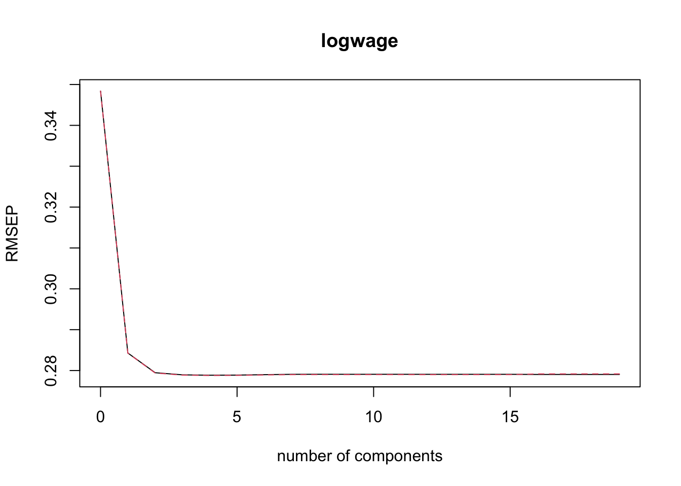
## Step 4: Identify the CV RMSE for the number of components with
## the lowest CV RMSE
pls_rmsep <- RMSEP(pls_fit)
print(pls_rmsep$val[1, 1, as.numeric(pls_min_indx)])
[1] 0.2788531## Step 5: Predict test set logwage values
pls_pred <- predict(pls_fit, wage_data[test,],
ncomp = (as.numeric(pls_min_indx) -1))
## Step 6: Measure test MSE and RMSE
pls_test_MSE <- mean((pls_pred - wage_data[test, "logwage"])^2)
print(pls_test_MSE)[1] 0.07881288print(sqrt(pls_test_MSE))[1] 0.2807363